Note
Go to the end to download the full example code.
Distribution#
Visualize state-occupancy distributions over time with
SequenceVisualizer.
Each time bin shows how many (or what fraction of) sequences occupy each state at that moment, using occupancy-based binning: a state segment contributes to every bin it overlaps.
Note
Compatible with state pools only.
Other pool types raise UnsupportedSequenceTypeError.
Imports#
import polars as pl

from tanat import build_states
from tanat.dataset import simulate_states, simulate_static
from tanat.visualization import SequenceVisualizer
Simulate data#
simulate_states() produces strictly
contiguous states (end[i] == start[i+1]). The second feature (status)
is categorical; it labels the occupancy areas.
temporal = simulate_states(
    n_ids=80,
    seq_length_range=(4, 12),
    features=["value", "status"],
    seed=42,
)
print(temporal.shape, temporal.columns.tolist())
(654, 5) ['id', 'start', 'end', 'value', 'status']
temporal.head()
Build the pool#
build_states() accepts an explicit end_column
when the data is already contiguous; simulate_states()
always guarantees.
pool = build_states(
    temporal_data=temporal,
    id_column="id",
    start_column="start",
    end_column="end",
)
┌─ State SequenceStore
│
│ Step 1/4: Sorting & preparing data
│
│ Step 2/4: Building sequence index
│
│ Step 3/4: Writing entity & time index features
│
│ Step 4/4: Computing & writing metadata
│
└─ Done (80 sequences · 654 entities · 0.00s)
pool.cast_features({"status": pl.Categorical}, is_static=False)
print(pool)
┌────────────────────────────────────────────────┐
│           StateSequencePool Summary            │
└────────────────────────────────────────────────┘

Overview
─────────────────────────
  Sequences          80
  Store              /home/runner/.tanat/_quick_state_682e89fe
  id_column          id

Time Index
─────────────────────────
  Type               Datetime(time_unit='us', time_zone=None) [2000-03-25 13:26:52.303819 → 2025-01-01 00:00:00]
  Columns            ['start', 'end']
  t0                 position=0, anchor=start

Entity Features (2)
─────────────────────────
  • status              Categorical (5 categories)
  • value               Numerical [1 → 100]
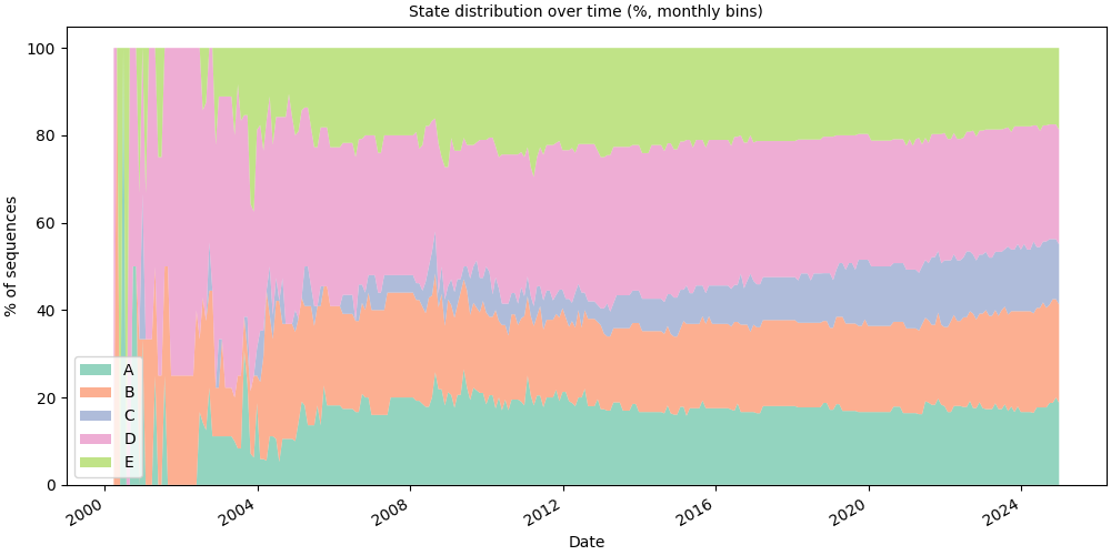
Default: percentage stacked area#
mode="percentage" (default) renders each state’s share summing to 100%
per bin, the classic state-sequence distribution chart.
# fmt: off
SequenceVisualizer.distribution(mode="percentage", bin_size="1mo") \
    .title("State distribution over time (%, monthly bins)") \
    .x_axis(label="Date", rotation=30, autofmt_xdate=True) \
    .y_axis(label="% of sequences") \
    .colors("Set2") \
    .draw(pool, entity_feature="status") \
    .show()
# fmt: on
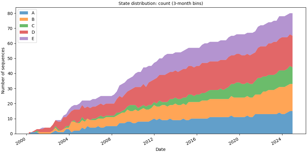
Modes: count, proportion, percentage#
|
y-axis |
Sum per bin |
|---|---|---|
|
raw number of sequences |
varies |
|
fraction (0–1) |
1.0 |
|
percent (0–100) |
100 |
# Raw counts
# fmt: off
SequenceVisualizer.distribution(mode="count", bin_size="3mo") \
    .title("State distribution: count (3-month bins)") \
    .x_axis(label="Date", rotation=30, autofmt_xdate=True) \
    .y_axis(label="Number of sequences") \
    .colors("tab10") \
    .draw(pool, entity_feature="status") \
    .show()
# fmt: on
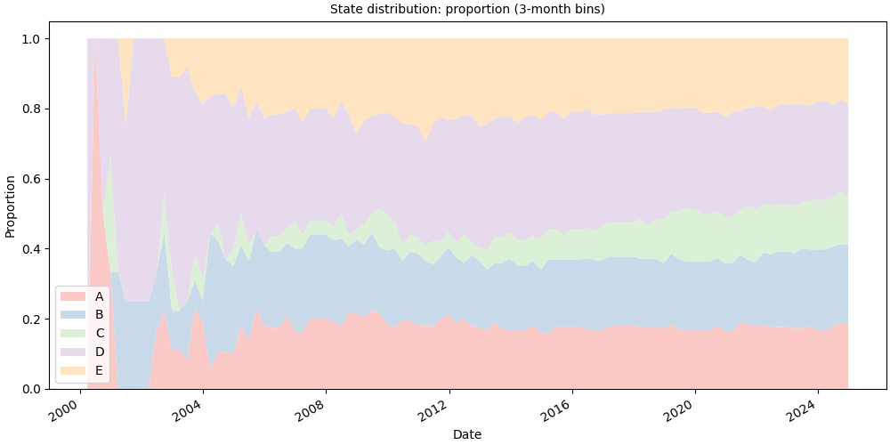
# Proportion (0-1 scale)
# fmt: off
SequenceVisualizer.distribution(mode="proportion", bin_size="3mo") \
    .title("State distribution: proportion (3-month bins)") \
    .x_axis(label="Date", rotation=30, autofmt_xdate=True) \
    .y_axis(label="Proportion") \
    .colors("Pastel1") \
    .draw(pool, entity_feature="status") \
    .show()
# fmt: on
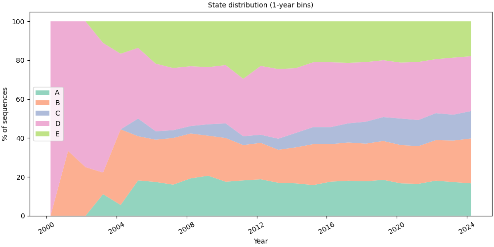
Bin size#
bin_size accepts any Polars duration string: "1d", "1w",
"1mo", "1y". Use coarser bins for long time horizons, finer
bins for detailed short-term patterns.
# Yearly bins, smoothest view for long horizons
# fmt: off
SequenceVisualizer.distribution(mode="percentage", bin_size="1y") \
    .title("State distribution (1-year bins)") \
    .x_axis(label="Year", rotation=30) \
    .y_axis(label="% of sequences") \
    .colors("Set2") \
    .draw(pool, entity_feature="status") \
    .show()
# fmt: on
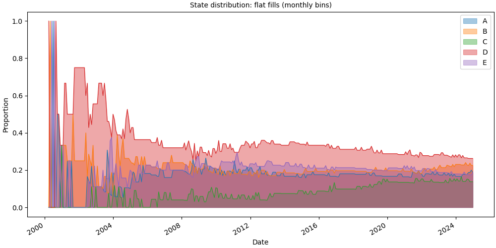
Flat (unstacked) fills#
stacked=False renders overlapping transparent fills, easier to compare
individual state curves without stacking artefacts.
# fmt: off
SequenceVisualizer.distribution(mode="proportion", bin_size="1mo", stacked=False) \
    .title("State distribution: flat fills (monthly bins)") \
    .x_axis(label="Date", rotation=30, autofmt_xdate=True) \
    .y_axis(label="Proportion") \
    .marker(alpha=0.4) \
    .colors("tab10") \
    .draw(pool, entity_feature="status") \
    .show()
# fmt: on
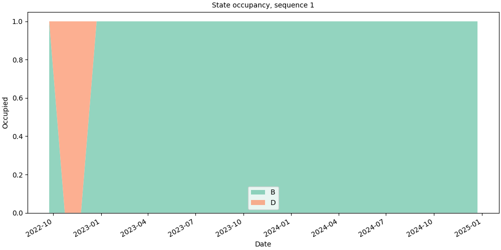
Single sequence#
Pass a Sequence directly to inspect
one individual’s state occupancy.
seq = pool[pool.unique_ids[0]]
print(f"ID {seq.id_value}: {len(seq)} states")
ID 1: 4 states
# fmt: off
SequenceVisualizer.distribution(mode="count", bin_size="1mo") \
    .title(f"State occupancy, sequence {seq.id_value}") \
    .x_axis(label="Date", rotation=30, autofmt_xdate=True) \
    .y_axis(label="Occupied") \
    .colors("Set2") \
    .draw(seq, entity_feature="status") \
    .show()
# fmt: on
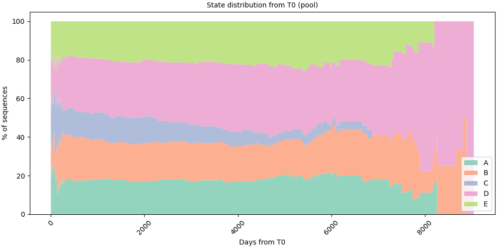
Relative time mode#
time_mode="relative" shifts every sequence so that T0 becomes the
origin of the x-axis (0 days). The axis then shows a numeric offset in
days, and bin_size retains its usual Polars duration meaning
(e.g. "1d" → one-day bins).
Call set_t0() to set the reference
point; without it the lazy default (position=0) is used.
Anchor T0 to the first state of every sequence.
pool.set_t0(position=0, anchor="start")
StateSequencePool(n=80, entity_features=2, static_features=0, store='/home/runner/.tanat/_quick_state_682e89fe')
# Pool: state distribution relative to each sequence's T0
# fmt: off
SequenceVisualizer.distribution(time_mode="relative", bin_size="1d") \
    .title("State distribution from T0 (pool)") \
    .x_axis(label="Days from T0") \
    .y_axis(label="% of sequences") \
    .colors("Set2") \
    .draw(pool, entity_feature="status") \
    .show()
# fmt: on
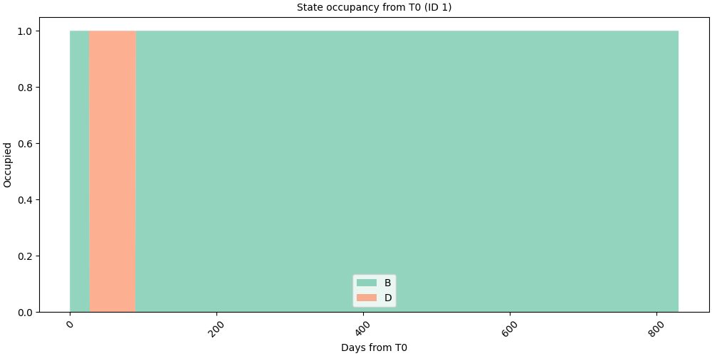
# Single sequence: occupancy relative to that individual's T0
# fmt: off
SequenceVisualizer.distribution(time_mode="relative", mode="count", bin_size="1d") \
    .title(f"State occupancy from T0 (ID {seq.id_value})") \
    .x_axis(label="Days from T0") \
    .y_axis(label="Occupied") \
    .colors("Set2") \
    .draw(seq, entity_feature="status") \
    .show()
# fmt: on
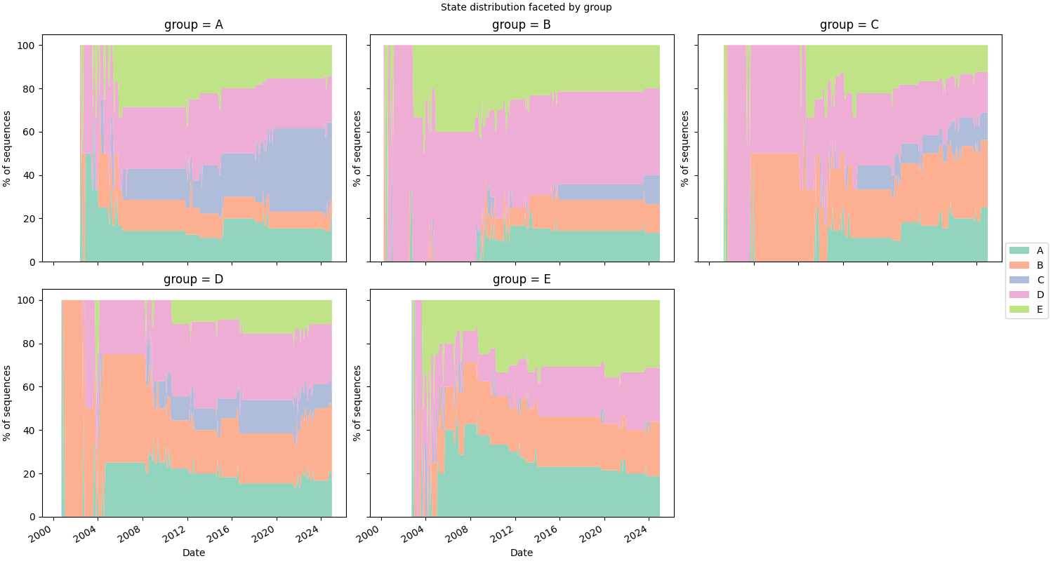
Faceting#
.facet() splits the chart into a grid of panels, one per unique value
of a chosen feature. Here we attach per-sequence static data and facet on
group.
static_df = simulate_static(n_ids=80, features=["age", "group"], seed=0)
pool.add_static_features(static_df)
pool.cast_features({"group": pl.Categorical}, is_static=True)
# fmt: off
SequenceVisualizer.distribution(mode="percentage", bin_size="1mo") \
    .facet(by="group", is_static=True, cols=3) \
    .title("State distribution faceted by group") \
    .x_axis(label="Date", rotation=30, autofmt_xdate=True) \
    .y_axis(label="% of sequences") \
    .colors("Set2") \
    .draw(pool, entity_feature="status") \
    .show()
# fmt: on
Inspect prepare_data()#
prepare_data() returns the binned Polars DataFrame before rendering.
Columns: __BIN__, __LABEL__, __VALUE__, and optionally __COLOR__.
builder = SequenceVisualizer.distribution(mode="percentage", bin_size="1mo")
df = builder.prepare_data(pool, entity_feature="status")
print(f"Shape: {df.shape}, schema: {dict(df.schema)}")
df.head(10)
Shape: (1377, 4), schema: {'__TIME_BIN__': Datetime(time_unit='us', time_zone=None), '__LABEL__': String, '__VALUE__': Float64, '__COLOR__': String}
Total running time of the script: (0 minutes 2.317 seconds)