
Note
Go to the end to download the full example code.
Exploring a patient cohort#
Scenario: You have access to the MIMIC-IV demo dataset, a subset of de-identified electronic health records from the Beth Israel Deaconess Medical Center. Each patient has a sequence of hospital admissions characterised by their type (emergency, elective, …) and admission location.
The goal of this tutorial is to load the data, build a TanaT pool, and perform an initial exploratory analysis.
Concepts covered:
Access the MIMIC-IV demo with
access()Ingest two SQL tables with the builder API into an
IntervalSequencePoolSummarise the pool with
describe()Navigate sequences and individual admissions
Visualise the admission-type distribution and individual timelines
Split into train / test with
train_test_split()
Note
MIMIC-IV data is downloaded automatically on first use and cached locally. The demo subset covers ~100 patients and is freely available via Zenodo.
Imports#
import polars as pl

from tanat.dataset import access
from tanat.sequence.type.interval.pool import IntervalSequencePool
from tanat.visualization import SequenceVisualizer
Load the MIMIC-IV demo#
access() downloads the SQLite database on the first
call and returns the local path. The builder API accepts SQL queries
directly, with no intermediate DataFrames. Two sources are chained:
hosp/admissions: one row per hospital stay (temporal, interval).hosp/patients: one row per patient (static features,is_static=True).
DB = f"sqlite:///{access('mimic4')}"

pool = IntervalSequencePool(
    store=(
        IntervalSequencePool.builder()
        .add_sql(
            DB,
            "SELECT subject_id, admittime, dischtime,"
            "       admission_type, admission_location"
            ' FROM "hosp/admissions"',
            id_column="subject_id",
            start_column="admittime",
            end_column="dischtime",
            features=["admission_type", "admission_location"],
        )
        .add_sql(
            DB,
            'SELECT subject_id, gender, anchor_age AS age FROM "hosp/patients"',
            id_column="subject_id",
            is_static=True,
            features=["gender", "age"],
        )
        .build("admissions_store", exist_ok=True)
    )
)

# ``pl.Categorical`` is required by the metric and clustering modules, and
# enables consistent colour-coding across all visualisations.
pool.cast_features({"admission_type": pl.Categorical}, is_static=False)
┌─ Interval SequenceStore
│
│ Step 1/4: Sorting & preparing data
│
│ Step 2/4: Building sequence index
│
│ Step 3/4: Writing entity, time index & static features
│
│ Step 4/4: Computing & writing metadata
│
└─ Done (100 sequences · 275 entities · 0.01s)
print(pool)
┌────────────────────────────────────────────────┐
│          IntervalSequencePool Summary          │
└────────────────────────────────────────────────┘

Overview
─────────────────────────
  Sequences          100
  Store              /home/runner/.tanat_workspace/building_pools_tutorial/admissions_store
  id_column          id

Time Index
─────────────────────────
  Type               Datetime(time_unit='us', time_zone=None) [2110-04-11 15:08:00 → 2201-12-17 13:45:00]
  Columns            ['start', 'end']
  t0                 position=0, anchor=start

Entity Features (2)
─────────────────────────
  • admission_location  String [len 4 → 38]
  • admission_type      Categorical (9 categories)

Static Features (2)
─────────────────────────
  • age                 String [len 2 → 2]
  • gender              String [len 1 → 1]
Describe the cohort#
describe() summarises the pool.
by_id=False returns aggregate statistics across all patients;
by_id=True returns one row per patient.
pool.describe(by_id=False)
pool.describe(by_id=True).head()
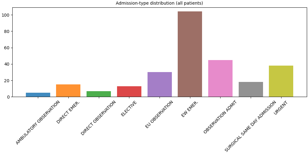
Distribution of admission types#
A barplot gives a quick overview of how often each admission type appears across the full cohort.
# fmt: off
SequenceVisualizer.barplot() \
    .title("Admission-type distribution (all patients)") \
    .colors("tab10") \
    .draw(pool, entity_feature="admission_type") \
    .show()
# fmt: on
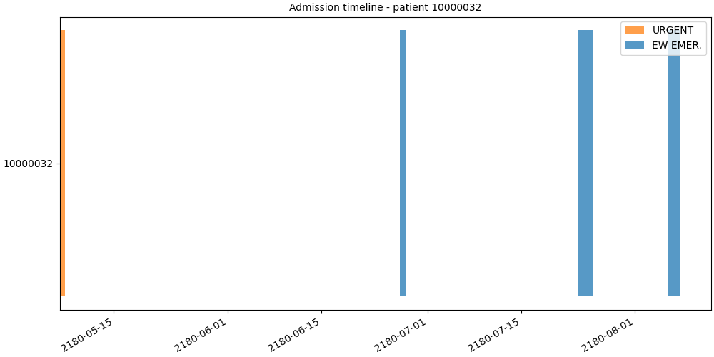
Individual patient timeline#
Indexing the pool by a patient ID returns a
Sequence whose admissions can be
rendered as a horizontal timeline.
pid = pool.unique_ids[0]
seq = pool[pid]

print(f"Patient {pid}: {len(seq)} admissions")
print(seq.temporal_data())
Patient 10000032: 4 admissions
         id                start  ...      admission_location admission_type
0  10000032  2180-05-06 22:23:00  ...  TRANSFER FROM HOSPITAL         URGENT
1  10000032  2180-06-26 18:27:00  ...          EMERGENCY ROOM       EW EMER.
2  10000032  2180-07-23 12:35:00  ...          EMERGENCY ROOM       EW EMER.
3  10000032  2180-08-05 23:44:00  ...          EMERGENCY ROOM       EW EMER.

[4 rows x 5 columns]
# fmt: off
SequenceVisualizer.timeline() \
    .title(f"Admission timeline - patient {pid}") \
    .colors("tab10") \
    .draw(seq, entity_feature="admission_type") \
    .show()
# fmt: on
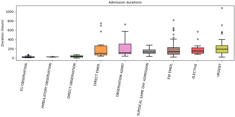
Explore duration of admissions#
A span plot shows the duration of each admission type as a box plot. This reveals which admission types tend to be short (e.g. observation) vs. long (e.g. elective surgery).
# fmt: off
SequenceVisualizer.spanplot(display_unit="hours") \
    .title("Admission durations") \
    .colors("tab10") \
    .x_axis(rotation=80) \
    .y_axis(label="Duration (hours)") \
    .draw(pool, entity_feature="admission_type") \
    .show()
# fmt: on
Train / test split#
train_test_split() splits at
the patient level for downstream predictive modelling.
train, test = pool.train_test_split(test_size=0.2, random_state=42)

print(f"Train : {len(train)} patients")
print(f"Test  : {len(test)} patients")
Train : 80 patients
Test  : 20 patients
Merging splits#
extend() merges two pools back
into one. Here we verify that the combined pool recovers all original patients.
extended = train.extend(test)
print(len(extended))
100
Total running time of the script: (0 minutes 0.958 seconds)