Discretizing time series into sequences

Time series is another type of temporal data that are often encountered, and there are already many libraries that are dedicated to the analysis of such type of data, for instance the aeon toolkit or sktime.

In this tutorial, we illustrate the complementarity between a library dedicated to time series, and TanaT dedicated to the analysis of temporal sequences. More specifically, time series segmentation is a machine learning task that bridges the two worlds. It identifies contiguous regions of a time series with a consistent behavior. The segmentation output is a kind of a sequence state that can be further analyzed (for example, by clustering).

Note

aeon is not bundled with TanaT. Install it separately:

pip install aeon

Concepts covered:

• Create a pool of state sequence

• Visualization of TanaT and combination with additional plots

some generic imports

import pandas as pd
import polars as pl
import numpy as np

from tanat import build_events
from tanat.visualization import SequenceVisualizer

Prepare some simulated time series data

Create a dataset of time series with aeon The load_unit_test creates time series between 0 and 1000. Scaling values between 0 and 1 fits better the processings to follow.

from aeon.datasets import load_unit_test

X_raw, _ = load_unit_test()
X_raw = X_raw.squeeze() / 1000

Create a simple symbolic representation

A first naive approach for transforming time series as sequences is to use the discretization technique named SAX, which discretize the time and assign a symbol to each segment based on its mean value.

The object that is obtained is a sequence of states, suitable for TanaT.

from aeon.transformations.collection.dictionary_based import SAX

n_segments = 10
voc_size = 15

sax = SAX(n_segments=n_segments, alphabet_size=voc_size)

X_sax = sax.fit_transform(X_raw).squeeze()

We obtain a sequence of symbols (a symbol is coded by an integer)

print(X_sax)

[[ 9  8  7  9 13 13 12 12 11  9]
 [ 9  8  7  9 13 13 13 13 11 10]
 [ 9  8  7 10 13 13 13 13 11  8]
 [ 9  7  7 10 13 13 13 14 13 11]
 [ 9  7  7  9 12 12 12 12 11 10]
 [ 9  7  7  9 13 13 12 12 11  9]
 [ 9  8  8  9 13 13 13 13 13 12]
 [ 9  7  8 10 14 14 14 14 13 12]
 [ 9  8  8 10 13 13 13 14 14 13]
 [ 9  8  7  9 13 13 13 14 13 12]
 [ 7  7  8  9 13 13 13 13 12 10]
 [ 8  7  8  9 13 12 12 14 13 11]
 [ 7  7  8  9 12 11 12 13 11  9]
 [ 7  7  8 10 13 12 12 13 12  9]
 [ 8  7  8 10 13 12 13 14 13 11]
 [ 8  7  7 10 13 13 13 13 12  9]
 [ 7  7  8 10 13 12 12 13 11  9]
 [ 7  7  8  9 12 12 12 13 12  9]
 [ 7  7  8  9 13 13 12 13 11  9]
 [ 7  7  8  9 13 12 12 12 10  8]
 [ 9  8  7 10 13 13 13 13 11  9]
 [12 10  8  9 12 12 12 12 11  9]
 [ 9  7  7 10 13 13 13 14 13 12]
 [ 9  8  7 12 14 14 14 13 12  9]
 [ 9  7  7  9 12 12 12 12 12 11]
 [ 9  8  7  9 13 13 13 14 13 12]
 [ 9  7  8  9 13 13 13 14 13 11]
 [ 9  7  7  9 13 13 13 14 13 11]
 [ 9  7  7  9 13 13 13 14 13 12]
 [ 9  8  8 10 13 13 13 14 12 11]
 [ 9  8  7 10 13 13 13 13 12 10]
 [ 9  7  7 10 13 13 13 14 13 11]
 [ 8  7  8  9 12 11 12 12 12 10]
 [ 8  7  8  9 13 12 12 13 12 11]
 [ 8  7  7 10 14 13 13 13 13 11]
 [ 8  7  8  9 12 11 12 13 12 11]
 [ 7  7  8 10 13 13 12 12 11  9]
 [ 9  8  7 10 14 13 13 14 13 11]
 [ 7  7  8  9 12 12 12 13 12  9]
 [ 7  7  8  9 13 11 12 12 10  8]
 [ 7  7  8  9 13 13 12 13 11  9]
 [ 8  7  7  9 13 13 12 12 11  9]]

Let us transform the results as a pandas dataframe ready for TanaT

values = [
    (seq, t, X_sax[seq, t]) for seq in range(X_raw.shape[0]) for t in range(n_segments)
]
df = pd.DataFrame(values, columns=["id", "t", "value"])

It can now be ingested by TanaT as a pool of event sequences Here, we choose to create a pool of events and then to convert it as a pool of state sequences.

pool = build_events(df, id_column="id", time_column="t")
state_pool = pool.as_state(end_value=11)
state_pool.cast_features({"value": pl.String})
state_pool.cast_features({"value": pl.Categorical})

┌─ Event SequenceStore
│
│ Step 1/4: Sorting & preparing data
│
│ Step 2/4: Building sequence index
│
│ Step 3/4: Writing entity & time index features
│
│ Step 4/4: Computing & writing metadata
│
└─ Done (42 sequences · 420 entities · 0.00s)

Note

We convert the value feature as Categorical for the visualisation of sequences. Direct convertion from integer to Categorical throw an error, the reason why we convert first the values as string.

print(state_pool)

┌────────────────────────────────────────────────┐
│           StateSequencePool Summary            │
└────────────────────────────────────────────────┘

Overview
─────────────────────────
  Sequences          42
  Store              /home/runner/.tanat_workspace/building_pools_tutorial/_quick_event_cff0402e
  id_column          id

Time Index
─────────────────────────
  Type               Int64 (Timestep) [0 → 11]
  Columns            ['start', 'end']
  t0                 position=0, anchor=None

Entity Features (1)
─────────────────────────
  • value               Categorical (8 categories)

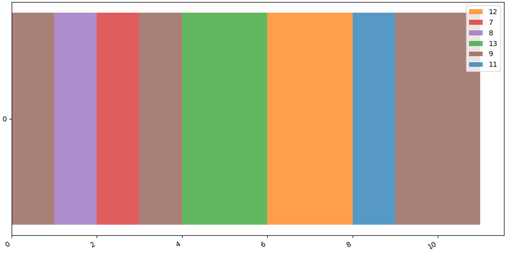
Let us illustrate one of the sequence

ts_id = 0  # identifier of the time-series / sequence to show
seq = state_pool[ts_id]
SequenceVisualizer.timeline().draw(seq, entity_feature="value").show()

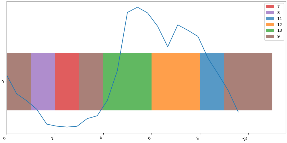
We can also overlay the original time series on the TanaT visualization. The x-axis is rescaled to align with the SAX timestamps, and the values are shifted by $-0.5$ to center the curve within the symbolic view.

figres = SequenceVisualizer.timeline().draw(seq, entity_feature="value")
figres.figure.axes[0].plot(
    np.arange(X_sax.shape[1], step=X_sax.shape[1] / X_raw.shape[1]), X_raw[ts_id] - 0.5
)
figres.show()