Note
Go to the end to download the full example code.
Timeline#
Visualize a Sequence or SequencePool
as a timeline using SequenceVisualizer.
Each row spans [start, end] for interval and state pools (horizontal bars);
event pools render as scatter points. Two row-organisation modes are available:
group_by="id": one row per sequence (default, up to 30 sequences)group_by="category": one row per unique label value
Imports#
import polars as pl

from tanat import build_events, build_intervals
from tanat.dataset import simulate_events, simulate_intervals, simulate_static
from tanat.visualization import SequenceVisualizer
Simulate data#
simulate_intervals() produces one row
per interval. The second feature (status) is categorical; it becomes the
label rendered on the timeline.
temporal = simulate_intervals(
    n_ids=20,
    seq_length_range=(4, 10),
    features=["value", "status"],
    seed=42,
)
print(temporal.shape, temporal.columns.tolist())
(146, 5) ['id', 'start', 'end', 'value', 'status']
temporal.head()
Build the pool#
pool = build_intervals(
    temporal_data=temporal,
    id_column="id",
    start_column="start",
    end_column="end",
)
┌─ Interval SequenceStore
│
│ Step 1/4: Sorting & preparing data
│
│ Step 2/4: Building sequence index
│
│ Step 3/4: Writing entity & time index features
│
│ Step 4/4: Computing & writing metadata
│
└─ Done (20 sequences · 146 entities · 0.00s)
pool.cast_features({"status": pl.Categorical}, is_static=False)
print(pool)
┌────────────────────────────────────────────────┐
│          IntervalSequencePool Summary          │
└────────────────────────────────────────────────┘

Overview
─────────────────────────
  Sequences          20
  Store              /home/runner/.tanat/_quick_interval_3a2a5e3d
  id_column          id

Time Index
─────────────────────────
  Type               Datetime(time_unit='us', time_zone=None) [2000-02-19 14:02:45.190748 → 2024-12-31 19:24:06.829108]
  Columns            ['start', 'end']
  t0                 position=0, anchor=start

Entity Features (2)
─────────────────────────
  • status              Categorical (5 categories)
  • value               Numerical [1 → 100]
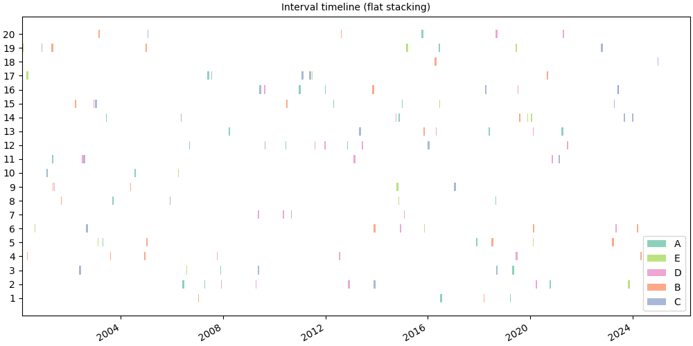
Flat timeline: one row per sequence#
group_by="id" (default) assigns one horizontal band per sequence.
Each bar spans the [start, end] of that interval.
# fmt: off
SequenceVisualizer.timeline() \
    .title("Interval timeline (flat stacking)") \
    .colors("Set2") \
    .draw(pool, entity_feature="status") \
    .show()
# fmt: on
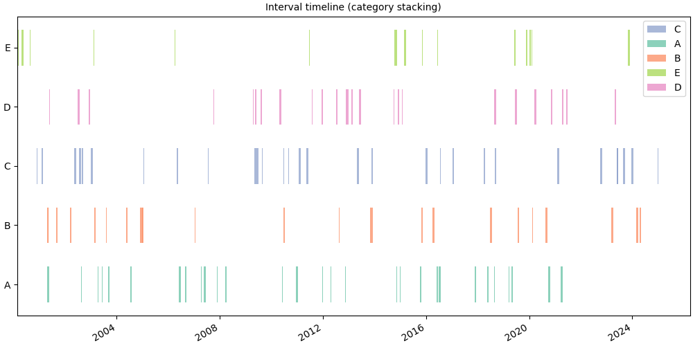
Category stacking: one row per label#
group_by="category" collapses all sequences onto one row per unique label
value. Useful to compare when each label is active across the time axis.
# fmt: off
SequenceVisualizer.timeline(group_by="category") \
    .title("Interval timeline (category stacking)") \
    .colors("Set2") \
    .draw(pool, entity_feature="status") \
    .show()
# fmt: on
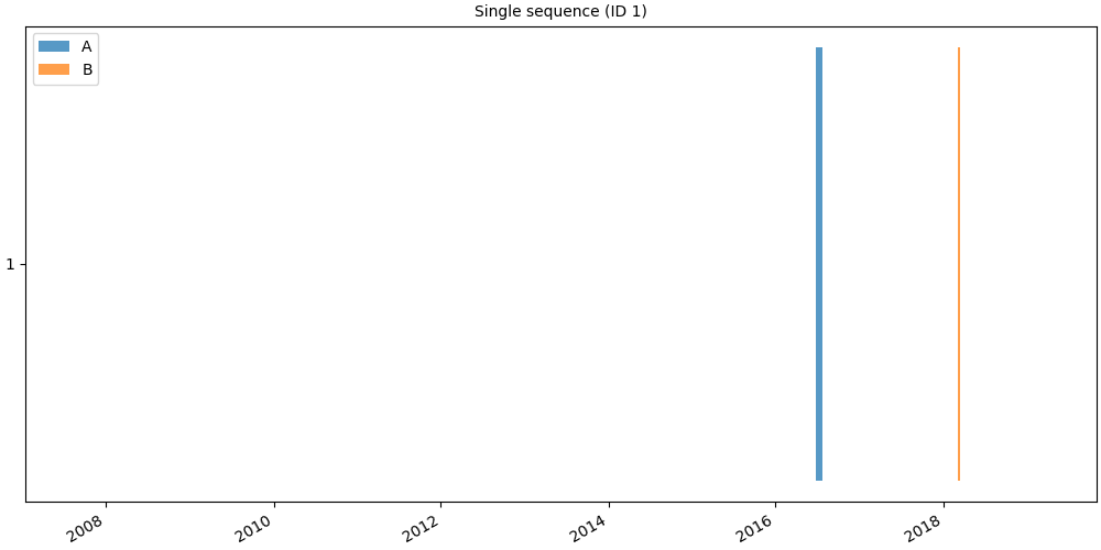
Single sequence#
Pass a Sequence directly for a per-individual view.
seq = pool[pool.unique_ids[0]]
print(f"ID {seq.id_value}: {len(seq)} intervals")
ID 1: 4 intervals
# fmt: off
SequenceVisualizer.timeline() \
    .title(f"Single sequence (ID {seq.id_value})") \
    .colors("tab10") \
    .draw(seq, entity_feature="status") \
    .show()
# fmt: on
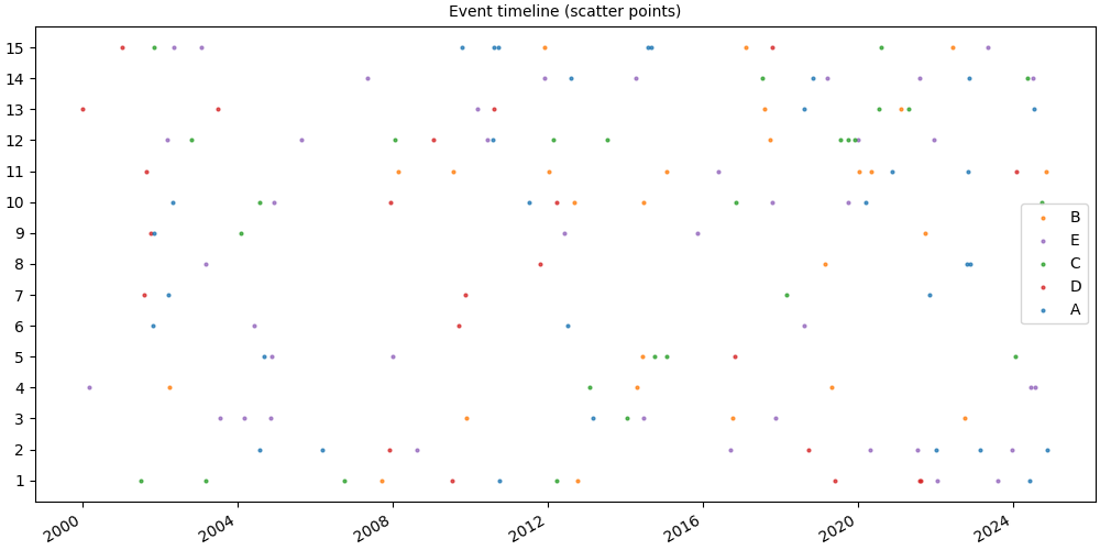
Event pool: scatter points#
For event pools (point observations) the timeline renders scatter marks instead of horizontal bars.
event_temporal = simulate_events(
    n_ids=15,
    seq_length_range=(5, 15),
    features=["score", "action"],
    seed=0,
)
event_pool = build_events(
    temporal_data=event_temporal,
    id_column="id",
    time_column="time",
)
┌─ Event SequenceStore
│
│ Step 1/4: Sorting & preparing data
│
│ Step 2/4: Building sequence index
│
│ Step 3/4: Writing entity & time index features
│
│ Step 4/4: Computing & writing metadata
│
└─ Done (15 sequences · 148 entities · 0.00s)
event_pool.cast_features({"action": pl.Categorical}, is_static=False)
print(event_pool)
┌────────────────────────────────────────────────┐
│           EventSequencePool Summary            │
└────────────────────────────────────────────────┘

Overview
─────────────────────────
  Sequences          15
  Store              /home/runner/.tanat/_quick_event_954425ef
  id_column          id

Time Index
─────────────────────────
  Type               Datetime(time_unit='us', time_zone=None) [2000-01-03 17:54:05.937674 → 2024-11-15 14:02:43.302235]
  Columns            ['time']
  t0                 position=0, anchor=None

Entity Features (2)
─────────────────────────
  • action              Categorical (5 categories)
  • score               Numerical [1 → 100]
# fmt: off
SequenceVisualizer.timeline() \
    .title("Event timeline (scatter points)") \
    .colors("tab10") \
    .draw(event_pool, entity_feature="action") \
    .show()
# fmt: on
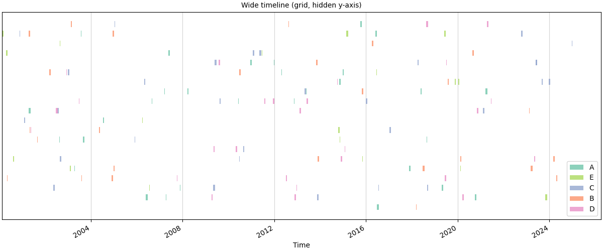
Layout and style#
# Wide figure with a grid, timestamps easier to read
# fmt: off
SequenceVisualizer.timeline() \
    .figsize(12, 5) \
    .grid() \
    .colors("Set2") \
    .x_axis(label="Time", autofmt_xdate=True) \
    .y_axis(show=False) \
    .title("Wide timeline (grid, hidden y-axis)") \
    .draw(pool, entity_feature="status") \
    .show()
# fmt: on
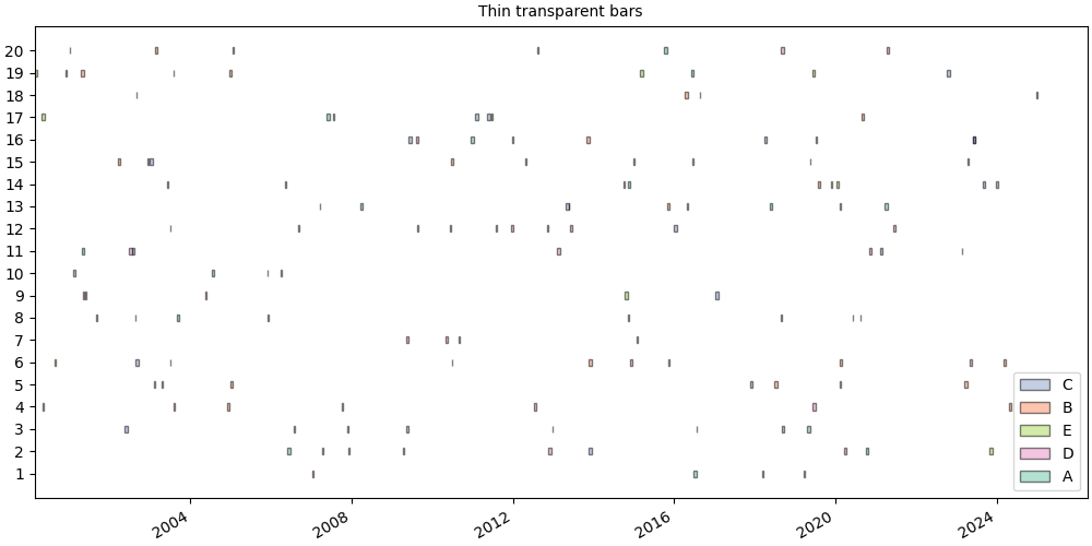
# Thin semi-transparent bars with a black edge
# fmt: off
SequenceVisualizer.timeline() \
    .colors("Set2") \
    .marker(bar_height=0.3, alpha=0.5, edge_color="black") \
    .title("Thin transparent bars") \
    .draw(pool, entity_feature="status") \
    .show()
# fmt: on
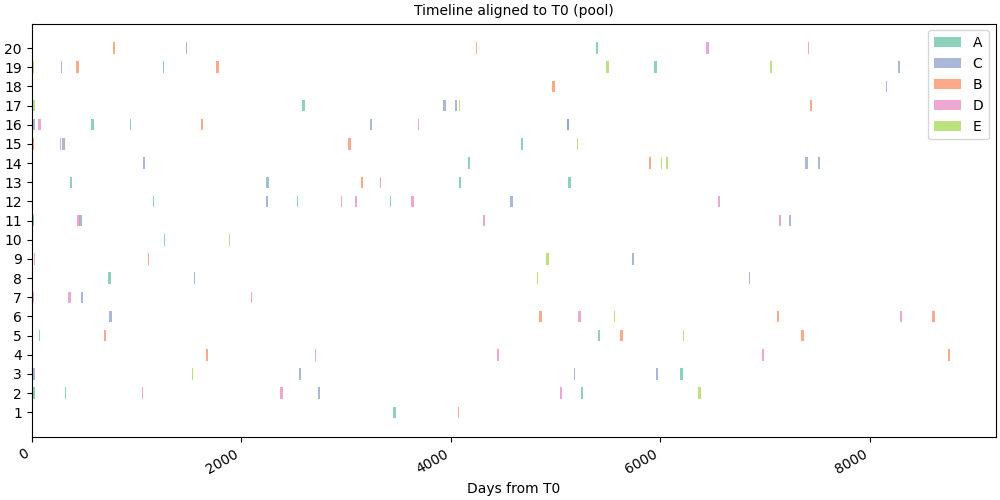
Relative time (aligned to T0)#
time_mode="relative" aligns every sequence to its own T0 reference
point so that the x-axis shows an offset in days from that anchor instead
of absolute timestamps. Call set_t0()
first to define the reference date; without it the lazy default
(position=0, i.e. the first row) is used.
Anchor T0 to the first interval of every sequence.
pool.set_t0(position=0, anchor="start")
IntervalSequencePool(n=20, entity_features=2, static_features=0, store='/home/runner/.tanat/_quick_interval_3a2a5e3d')
# Pool: all sequences aligned to their own t0
# fmt: off
SequenceVisualizer.timeline(time_mode="relative") \
    .title("Timeline aligned to T0 (pool)") \
    .x_axis(label="Days from T0") \
    .colors("Set2") \
    .draw(pool, entity_feature="status") \
    .show()
# fmt: on
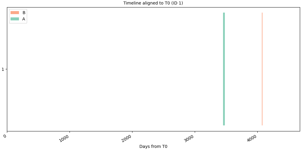
# Single sequence: the same shift applied to one individual
# fmt: off
SequenceVisualizer.timeline(time_mode="relative") \
    .title(f"Timeline aligned to T0 (ID {seq.id_value})") \
    .x_axis(label="Days from T0") \
    .colors("Set2") \
    .draw(seq, entity_feature="status") \
    .show()
# fmt: on
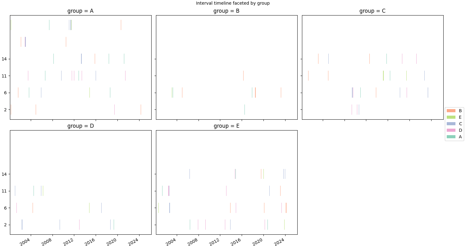
Faceting#
.facet() splits the chart into a grid of panels, one per unique value
of a chosen feature. Here we attach per-sequence static data and facet on
group.
static_df = simulate_static(n_ids=20, features=["age", "group"], seed=0)
pool.add_static_features(static_df)
pool.cast_features({"group": pl.Categorical}, is_static=True)
# fmt: off
SequenceVisualizer.timeline() \
    .facet(by="group", is_static=True, cols=3) \
    .title("Interval timeline faceted by group") \
    .colors("Set2") \
    .draw(pool, entity_feature="status") \
    .show()
# fmt: on
Inspect prepare_data()#
prepare_data() exposes the intermediate Polars DataFrame before rendering.
Columns: __ID__, __Y_POSITION__, __TIME__, __END__,
__LABEL__, and optionally __COLOR__.
builder = SequenceVisualizer.timeline(group_by="category").colors("Set2")
df = builder.prepare_data(pool, entity_feature="status")
df.head(10)
Total running time of the script: (0 minutes 2.413 seconds)