Analysing and clustering cohort sequences

Scenario: Starting from the cohort prepared in Filtering and preparing a cohort, you want to quantify how similar the admission sequences are across patients, group them into clusters with shared patterns, and visualise the results.

Concepts covered:

• Compute a pairwise sequence distance matrix with HammingEntityMetric + LinearPairwiseSequenceMetric

• Cluster with HierarchicalClusterer

• Inspect cluster membership

• Produce a faceted timeline coloured by cluster

Imports

import polars as pl

from tanat.clustering import HierarchicalClusterer
from tanat.criterion import (
    EntityCriterion,
    LengthCriterion,
)
from tanat.dataset import access
from tanat.metric import HammingEntityMetric, LinearPairwiseSequenceMetric
from tanat.sequence.type.interval.pool import IntervalSequencePool
from tanat.visualization import SequenceVisualizer

Rebuild the prepared cohort

Self-contained rebuild using the builder API (see Exploring a patient cohort and Filtering and preparing a cohort for details).

DB = f"sqlite:///{access('mimic4')}"

pool = IntervalSequencePool(
    store=(
        IntervalSequencePool.builder()
        .add_sql(
            DB,
            "SELECT subject_id, admittime, dischtime,"
            "       admission_type, admission_location"
            ' FROM "hosp/admissions"',
            id_column="subject_id",
            start_column="admittime",
            end_column="dischtime",
            features=["admission_type", "admission_location"],
        )
        .add_sql(
            DB,
            'SELECT subject_id, gender, anchor_age AS age FROM "hosp/patients"',
            id_column="subject_id",
            is_static=True,
            features=["gender", "age"],
        )
        .build("admissions_store", exist_ok=True)
    )
)
# ``pl.Categorical`` is required by the metric and clustering modules, and
# enables consistent colour-coding across all visualisations.
pool.cast_features({"admission_type": pl.Categorical}, is_static=False)

┌─ Interval SequenceStore
│
│ Step 1/4: Sorting & preparing data
│
│ Step 2/4: Building sequence index
│
│ Step 3/4: Writing entity, time index & static features
│
│ Step 4/4: Computing & writing metadata
│
└─ Done (100 sequences · 275 entities · 0.01s)

print(pool)

┌────────────────────────────────────────────────┐
│          IntervalSequencePool Summary          │
└────────────────────────────────────────────────┘

Overview
─────────────────────────
  Sequences          100
  Store              /home/runner/.tanat_workspace/building_pools_tutorial/admissions_store
  id_column          id

Time Index
─────────────────────────
  Type               Datetime(time_unit='us', time_zone=None) [2110-04-11 15:08:00 → 2201-12-17 13:45:00]
  Columns            ['start', 'end']
  t0                 position=0, anchor=start

Entity Features (2)
─────────────────────────
  • admission_location  String [len 4 → 38]
  • admission_type      Categorical (9 categories)

Static Features (2)
─────────────────────────
  • age                 String [len 2 → 2]
  • gender              String [len 1 → 1]

Cohort selection

Same selection as Filtering and preparing a cohort: patients with at least 2 admissions who experienced at least one emergency, aligned to their first emergency (T0).

ids_cohort = pool.which(LengthCriterion(ge=2)) & pool.which(
    EntityCriterion(query=pl.col("admission_type") == "EW EMER.")
)
print(f"[Intersection]      → {len(ids_cohort)} IDs")

[which]           LengthCriterion → 48 / 100 IDs (48.0%)
[which]           EntityCriterion → 60 / 100 IDs (60.0%)
[Intersection]      → 36 IDs

cohort = pool.subset(ids_cohort)
# Align sequences to first emergency admission (T0).
cohort.set_t0(query=pl.col("admission_type") == "EW EMER.", anchor="start")
print(cohort)

┌────────────────────────────────────────────────┐
│          IntervalSequencePool Summary          │
└────────────────────────────────────────────────┘

Overview
─────────────────────────
  Sequences          36
  Store              /home/runner/.tanat_workspace/building_pools_tutorial/admissions_store
  id_column          id

Time Index
─────────────────────────
  Type               Datetime(time_unit='us', time_zone=None) [2114-03-19 20:05:00 → 2201-12-17 13:45:00]
  Columns            ['start', 'end']
  t0                 query, anchor=start

Entity Features (2)
─────────────────────────
  • admission_location  String [len 4 → 38]
  • admission_type      Categorical (9 categories)

Static Features (2)
─────────────────────────
  • age                 String [len 2 → 2]
  • gender              String [len 1 → 1]

Step 1: Define the sequence metric

HammingEntityMetric compares two admissions at the same position: distance 0 if they share the same type, 1 otherwise. LinearPairwiseSequenceMetric aggregates these entity-level distances along the full sequence. The padding_penalty penalises sequences of different lengths.

entity_metric = HammingEntityMetric(entity_feature="admission_type")
sequence_metric = LinearPairwiseSequenceMetric(
    entity_metric=entity_metric,
    padding_penalty=1.0,
)

Step 2: Compute the distance matrix

dist_matrix = sequence_metric.compute_matrix(cohort)

┌─ LinearPairwiseSequenceMetric
│

│ Chunks:   0%|          | 0/1 [00:00<?, ?it/s]
│ Chunks: 100%|██████████| 1/1 [00:00<00:00, 5256.02it/s]
│
└─ Done (36 sequences · 0.00s)

dm = dist_matrix.data
print(f"Distance matrix shape : {dist_matrix.shape}")

Distance matrix shape : (36, 36)

Step 3: Hierarchical clustering

We group patients into 3 clusters using complete-linkage hierarchical clustering. After fit(), the cluster label is automatically added as a static feature on the pool under the name given by cluster_column.

clusterer = HierarchicalClusterer(
    metric=sequence_metric,
    n_clusters=3,
    linkage="complete",
    cluster_column="adm_cluster",
)
clusterer.fit(cohort)

┌─ HierarchicalClusterer
│
│ Step 1/2: Computing distance matrix
│
│   ┌─ LinearPairwiseSequenceMetric
│   │

│   │ Chunks:   0%|          | 0/1 [00:00<?, ?it/s]
│   │ Chunks: 100%|██████████| 1/1 [00:00<00:00, 5377.31it/s]
│   │
│   └─ Done (36 sequences · 0.00s)
│
│ Step 2/2: Clustering (HierarchicalClusterer)
│
└─ Done (36 items, 3 clusters · 0.02s)

HierarchicalClusterer(clusters=3)

Step 4: Inspect cluster membership

clusters exposes the fitted Cluster objects directly. Each provides a size and the list of patient items. The cluster label is also available as a static feature (adm_cluster) for downstream filtering or visualisation.

for cluster in clusterer.clusters:
    print(cluster)

Cluster(id=0, size=19)
Cluster(id=1, size=7)
Cluster(id=2, size=10)

Cluster labels are also stored as a static feature for downstream use.

cohort.static_data().head()

	id	adm_cluster	age	gender
0	10000032	0	52	F
1	10001217	2	55	F
2	10002428	1	80	F
3	10002930	1	48	F
4	10003400	1	72	F

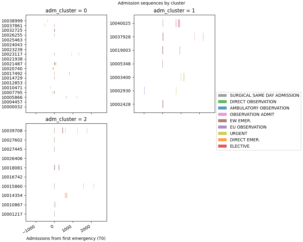
Step 5: Faceted timeline coloured by cluster

Each panel shows the admission sequences of one cluster, aligned to T0. This makes it easy to spot structural differences between groups.

fmt: off

SequenceVisualizer.timeline(time_mode="relative", allow_large=True) \
    .title("Admission sequences by cluster") \
    .x_axis(label="Admissions from first emergency (T0)") \
    .colors("tab10") \
    .facet(by="adm_cluster", is_static=True, cols=2, share_y=False) \
    .draw(cohort, entity_feature="admission_type") \
    .show()
# fmt: on