Survival analysis from cohort clusters

Scenario: Building on the clusters identified in Analysing and clustering cohort sequences, you want to ask whether patients in different admission clusters have different survival profiles. This tutorial shows how to build a time-to-event target with survival_target() and plot Kaplan-Meier curves for each cluster.

Concepts covered:

• Enrich an existing pool with a new static column via add_static_features()

• Inspect the survival target in pandas format before modelling with survival_target()

• Build a structured sksurv-compatible target

• Plot per-cluster Kaplan-Meier curves with sksurv and matplotlib

Imports

import pandas as pd
import matplotlib.pyplot as plt
import polars as pl
from sksurv.nonparametric import kaplan_meier_estimator

from tanat.clustering import HierarchicalClusterer
from tanat.criterion import EntityCriterion, LengthCriterion
from tanat.dataset import access
from tanat.metric import HammingEntityMetric, LinearPairwiseSequenceMetric
from tanat.sequence.type.interval.pool import IntervalSequencePool

Rebuild the cohort

We reuse the same admissions_store built in Exploring a patient cohort and Analysing and clustering cohort sequences.

DB_PATH = access("mimic4")
DB = f"sqlite:///{DB_PATH}"

pool = IntervalSequencePool(
    store=(
        IntervalSequencePool.builder()
        .add_sql(
            DB,
            "SELECT subject_id, admittime, dischtime,"
            "       admission_type, admission_location"
            ' FROM "hosp/admissions"',
            id_column="subject_id",
            start_column="admittime",
            end_column="dischtime",
            features=["admission_type", "admission_location"],
        )
        .add_sql(
            DB,
            'SELECT subject_id, gender, anchor_age AS age FROM "hosp/patients"',
            id_column="subject_id",
            is_static=True,
            features=["gender", "age"],
        )
        .build("admissions_store", exist_ok=True)
    )
)
# ``pl.Categorical`` is required by the metric and clustering modules, and
# enables consistent colour-coding across all visualisations.
pool.cast_features({"admission_type": pl.Categorical}, is_static=False)

┌─ Interval SequenceStore
│
│ Step 1/4: Sorting & preparing data
│
│ Step 2/4: Building sequence index
│
│ Step 3/4: Writing entity, time index & static features
│
│ Step 4/4: Computing & writing metadata
│
└─ Done (100 sequences · 275 entities · 0.01s)

print(pool)

┌────────────────────────────────────────────────┐
│          IntervalSequencePool Summary          │
└────────────────────────────────────────────────┘

Overview
─────────────────────────
  Sequences          100
  Store              /home/runner/.tanat_workspace/building_pools_tutorial/admissions_store
  id_column          id

Time Index
─────────────────────────
  Type               Datetime(time_unit='us', time_zone=None) [2110-04-11 15:08:00 → 2201-12-17 13:45:00]
  Columns            ['start', 'end']
  t0                 position=0, anchor=start

Entity Features (2)
─────────────────────────
  • admission_location  String [len 4 → 38]
  • admission_type      Categorical (9 categories)

Static Features (2)
─────────────────────────
  • age                 String [len 2 → 2]
  • gender              String [len 1 → 1]

Cohort selection, T0 alignment, and clustering

Same pipeline as Filtering and preparing a cohort and Analysing and clustering cohort sequences: patients with at least 2 admissions who had at least one emergency, aligned to their first emergency, then grouped into 3 clusters.

# Define the study cohort and align to T0.
ids_cohort = pool.which(LengthCriterion(ge=2)) & pool.which(
    EntityCriterion(query=pl.col("admission_type") == "EW EMER.")
)
print(f"Selected {len(ids_cohort)} patients for the cohort.")

[which]           LengthCriterion → 48 / 100 IDs (48.0%)
[which]           EntityCriterion → 60 / 100 IDs (60.0%)
Selected 36 patients for the cohort.

cohort = pool.subset(ids_cohort)
cohort.set_t0(query=pl.col("admission_type") == "EW EMER.", anchor="start")
print(cohort)

┌────────────────────────────────────────────────┐
│          IntervalSequencePool Summary          │
└────────────────────────────────────────────────┘

Overview
─────────────────────────
  Sequences          36
  Store              /home/runner/.tanat_workspace/building_pools_tutorial/admissions_store
  id_column          id

Time Index
─────────────────────────
  Type               Datetime(time_unit='us', time_zone=None) [2114-03-19 20:05:00 → 2201-12-17 13:45:00]
  Columns            ['start', 'end']
  t0                 query, anchor=start

Entity Features (2)
─────────────────────────
  • admission_location  String [len 4 → 38]
  • admission_type      Categorical (9 categories)

Static Features (2)
─────────────────────────
  • age                 String [len 2 → 2]
  • gender              String [len 1 → 1]

# Cluster the cohort based on admission sequences.
entity_metric = HammingEntityMetric(entity_feature="admission_type")
sequence_metric = LinearPairwiseSequenceMetric(
    entity_metric=entity_metric, padding_penalty=1.0
)

clusterer = HierarchicalClusterer(
    metric=sequence_metric,
    n_clusters=3,
    linkage="complete",
    cluster_column="adm_cluster",
)
clusterer.fit(cohort)

┌─ HierarchicalClusterer
│
│ Step 1/2: Computing distance matrix
│
│   ┌─ LinearPairwiseSequenceMetric
│   │

│   │ Chunks:   0%|          | 0/1 [00:00<?, ?it/s]
│   │ Chunks: 100%|██████████| 1/1 [00:00<00:00, 5152.71it/s]
│   │
│   └─ Done (36 sequences · 0.00s)
│
│ Step 2/2: Clustering (HierarchicalClusterer)
│
└─ Done (36 items, 3 clusters · 0.01s)

HierarchicalClusterer(clusters=3)

Enrich the cohort with mortality data

dod (date of death) is not in the original store. We load it directly from SQLite using the standard library to handle SQLite’s empty-string representation of missing values, then attach it as a new static feature with add_static_features().

survival_target() will infer occurred automatically from dod.is_not_null().

import sqlite3

con = sqlite3.connect(DB_PATH)
dod_df = pd.read_sql('SELECT subject_id, dod FROM "hosp/patients"', con)
con.close()

# SQLite stores missing dates as empty strings, convert to NaT, then to datetime.
dod_df["dod"] = pd.to_datetime(dod_df["dod"].replace("", pd.NaT), errors="coerce")

cohort.add_static_features(dod_df, id_column="subject_id")

# Inspect pool with the new static feature.
print(cohort)

┌────────────────────────────────────────────────┐
│          IntervalSequencePool Summary          │
└────────────────────────────────────────────────┘

Overview
─────────────────────────
  Sequences          36
  Store              /home/runner/.tanat_workspace/building_pools_tutorial/admissions_store
  id_column          id

Time Index
─────────────────────────
  Type               Datetime(time_unit='us', time_zone=None) [2114-03-19 20:05:00 → 2201-12-17 13:45:00]
  Columns            ['start', 'end']
  t0                 query, anchor=start

Entity Features (2)
─────────────────────────
  • admission_location  String [len 4 → 38]
  • admission_type      Categorical (9 categories)

Static Features (4)
─────────────────────────
  • adm_cluster         Numerical [0 → 2]
  • age                 String [len 2 → 2]
  • dod                 Datetime(time_unit='ns', time_zone=None) [2116-07-05 00:00:00 → 2201-12-24 00:00:00]
  • gender              String [len 1 → 1]

Step 1: Inspect the survival target

survival_target() assembles a (occurred, time) pair for each patient:

• occurred: True if dod is not null (death observed within follow-up), False otherwise (censored).

• time: duration from T0 to death, or to the last recorded admission end for censored patients.

Using fmt="pandas" first lets you inspect the result before fitting any model.

survival_df, valid_ids = cohort.survival_target(
    endpoint_time="dod",
    fmt="pandas",
)
print(f"Patients with valid survival data: {len(valid_ids)}")
print(f"Observed deaths : {survival_df['occurred'].sum()}")
survival_df.head()

Patients with valid survival data: 36
Observed deaths : 17

	id	occurred	time
0	10000032	True	74 days 05:33:00
1	10001217	False	35 days 15:59:00
2	10002428	False	1556 days 04:33:00
3	10002930	True	2078 days 11:35:00
4	10003400	True	1183 days 21:35:00

Step 2: Per-cluster survival summary

A quick summary table combining cluster size, observed death count, and the proportion of censored patients.

rows = []
for cluster in clusterer.clusters:
    subset = cohort.subset(cluster.items)
    y, _ = subset.survival_target(endpoint_time="dod", fmt="sksurv")
    rows.append(
        {
            "cluster": cluster.id,
            "n_patients": cluster.size,
            "n_deaths": int(y["occurred"].sum()),
            "n_censored": int((~y["occurred"]).sum()),
        }
    )

pd.DataFrame(rows).sort_values("cluster").reset_index(drop=True)

	cluster	n_patients	n_deaths	n_censored
0	0	19	11	8
1	1	7	4	3
2	2	10	2	8

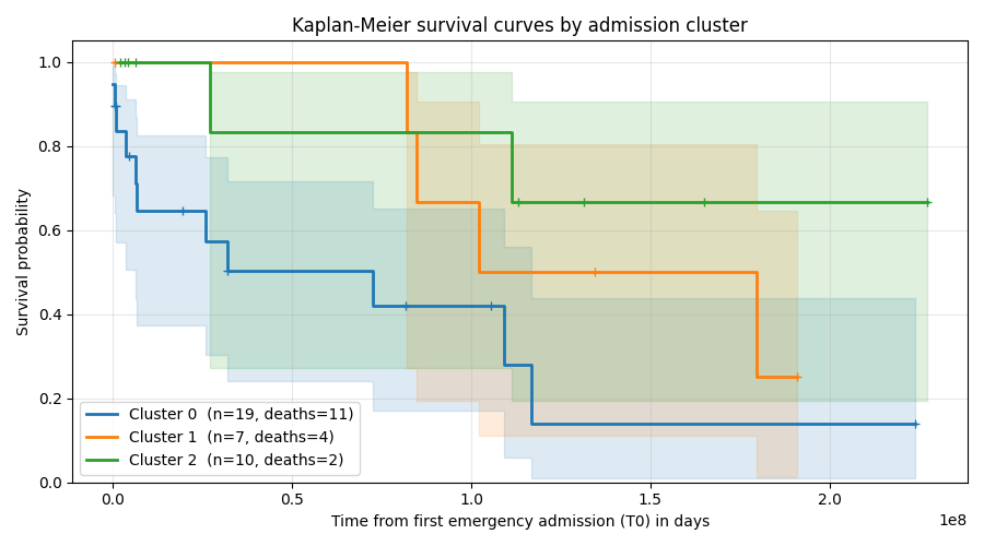
Step 3: Kaplan-Meier curves per cluster

We iterate over the 3 clusters, build a sksurv-compatible structured array with fmt="sksurv" for each subset, then plot the Kaplan-Meier estimator. Patients excluded by survival_target() (non-positive or unresolvable durations) are reported automatically via a warning. The shaded band is the 95 % log-log confidence interval; + tick marks indicate censored observations.

fig, ax = plt.subplots(figsize=(9, 5))
ax.set_prop_cycle(color=plt.cm.tab10.colors)

for cluster in clusterer.clusters:
    subset = cohort.subset(cluster.items)
    y, subset_ids = subset.survival_target(endpoint_time="dod", fmt="sksurv")

    time_points, survival_prob, conf_int = kaplan_meier_estimator(
        y["occurred"],
        y["time"].astype(float),
        conf_type="log-log",
    )
    conf_lower, conf_upper = conf_int
    (line,) = ax.step(
        time_points,
        survival_prob,
        where="post",
        linewidth=2,
        label=f"Cluster {cluster.id}  (n={cluster.size}, deaths={y['occurred'].sum()})",
    )
    # 95 % confidence band.
    ax.fill_between(
        time_points,
        conf_lower,
        conf_upper,
        step="post",
        alpha=0.15,
        color=line.get_color(),
    )
    # Mark censored observations with vertical ticks on the curve.
    censored_mask = ~y["occurred"]
    censored_times = y["time"][censored_mask].astype(float)
    # Interpolate survival probability at each censored time point.
    censored_probs = [
        float(survival_prob[time_points <= t][-1]) if (time_points <= t).any() else 1.0
        for t in censored_times
    ]
    ax.plot(
        censored_times,
        censored_probs,
        "+",
        color=line.get_color(),
        markersize=6,
    )

ax.set_title("Kaplan-Meier survival curves by admission cluster")
ax.set_xlabel("Time from first emergency admission (T0) in days")
ax.set_ylabel("Survival probability")
ax.set_ylim(0, 1.05)
ax.legend()
ax.grid(alpha=0.3)
plt.tight_layout()
plt.show()